Data
Data was input into R Studio using the formatting show below. PAH compounds were given the names x1, x2, ... x57 within R Studio to simplify the naming convention within the program language. All samples were measured in, or converted to, a nanogram/L concentration. The station name was prescribed following Alberta Environment and Park's naming convention XX##XX#### where:
- XX - province
- ##- continental river basin
- XX - sub basin
- #### - randomly assigned variables to describe the station.
Table 1. Sample data of PAH concentrations input into R Studio for analysis. Predictive parameters included the river (RVR), the sampling location (STN), and the sampling date and month. Sampling locations include the Ells (1), Tar (2), Muskeg (2), MacKay (2), and Steepbank (2) rivers. These stations are located up and downstream of industrial development. Dates are formatted as %Y-%b-%d and an additional column includes the month of the year.

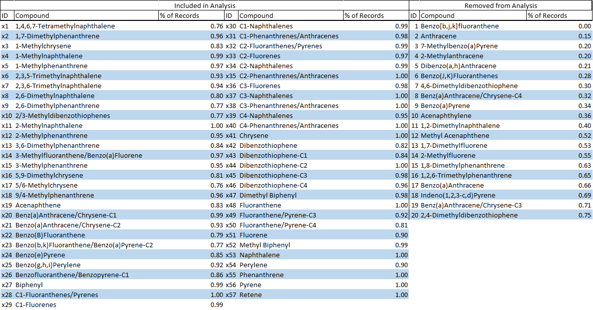
Table 2. Due to the complexity of organic chemistry naming conventions, names were substituted for sequential identifiers (X1, X2, ....) for ease of use in R programming language. PAH compound names and identifiers were tabulated for reference with their unique identifier.
Data Management
|
The raw data for the five rivers totals 1301 samples between 2015 and 2020. The data was cleaned for use in statistical analysis. There are 17 PAH surrogate recovery assessments for each grab sample. Where the average surrogate recovery was less than 50% or was not performed the sample was removed (see histograms to the right). Where more than 36 of the 77 parameters were non-detect, samples were removed. 20 of the 77 parameters were recorded in less than 75% of the samples and were removed from the analysis. This process was completed to achieve a dataset with more than 93% recorded parameters. Following these assessments, the dataset consisted of 901 grab samples. RandomForest was used in RStudio employing 10 iterations and 10,000 trees to impute missing non-detect values.
|

Figure 7. Histograms of PAH distributions. The first histogram shows the frequency of surrogate recovery >50%. The lower histogram shows the frequency of non detect concentrations within a sample. The red line on both indicates the bounding limit of data retention. Data below this line was censored.
|
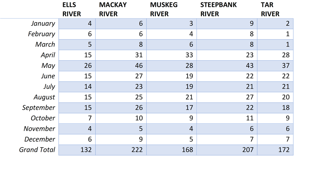
Table 3. Breakdown of the location and timing of all 901 samples included in analysis. Sample counts separated by river and month sampled. The strictest sampling program occurs during the summer months. However, surface water samples are taken throughout the year given safe conditions.
To ensure removal of samples with low surrogate recovery did not bias results data were plotted to ensure there were no obvious trends. Box and whisker plots of surrogate recovery distribution were compiled using the complete dataset. There were no obvious trends with recovery distribution. However surrogates X1, X2, X3, X9, and X15 had low medians near or below 50%.

Figure 8. Distribution of surrogate recoveries as Box and Whisker plots. This assessment shows no significant recovery bias based on PAH structure, or molecular weight.
|
Concentrations of PAHs were compared to surrogate recovery. This allowed for a rapid evaluation of potential bias (i.e. low surrogate recovery always aligned with low concentrations). The legend above remains the same for the charts on the right. As no trends were observed in these charts, removal of low recovery data mitigates a potential source of error without adding bias to the statistical analysis.
Due to the nature of these contaminants, there was a large range of values. To aid in visual analysis a Log+1 transformation was performed. This increased the visual effect of small deviations from the typical fractionation. Following discussion with a project lead, the data included some redundancy. Some PAHs compounds are included in the concentration measurements and sums of others. Following this discovery, a constrained analysis was performed on similarly structured PAHS incorporating different length hydrocarbon tails (i.e. C1-Naphthalenes, C2-Naphthalenes, C3-Naphthalenes, etc.). These different weights and structures are also a result of fractionation processes. The original ordinations of 55 hydrocarbons was nearly identical to an ordination of 13 compositional groups. |
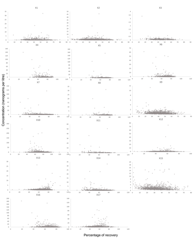
Figure 9. Scatter plots of surrogate recoveries. These plots were compiled to assess the bias between surrogate recovery and measured PAH concentrations. No bias requiring special assessment was observed.
|
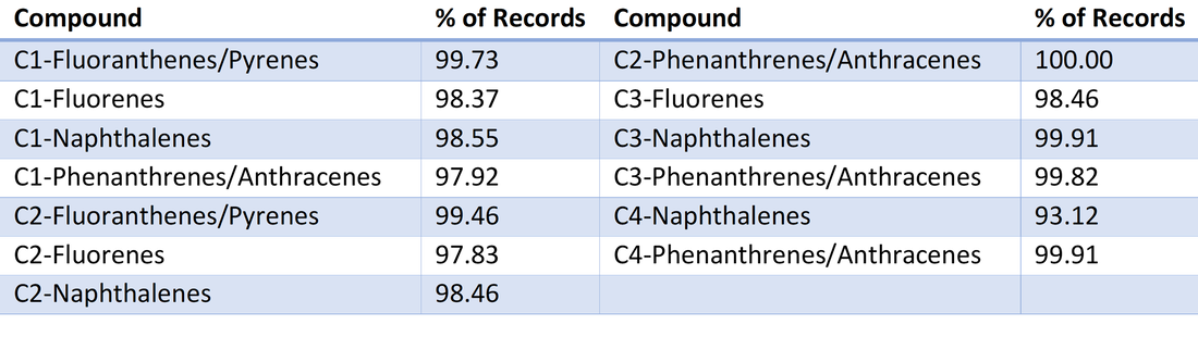
Table 4. List of compiled parameters used within the second ordination analysis. The additional chains on each structure affect the molecular weight and formation energy of each compound. This ordination produced a similar result and identical inferences as the ordination of the entire set of sampled compounds.
Principal coordinate analysis
Following the Log(x+1) transformation the data was scaled and Euclidean distances were calculated. A Mahalanobis distance calculation was attempted due to the likely autocorrelated nature of the fractionation process. However, the complete sampling set was too large for available computing power (>10gb memory require). The Mahalanobis distances of the smaller set yielded a much less clear ordination, but did show similar results. To ensure ordination results were comparable between both sample sets, Euclidean distances were used in the final analysis.
To reduce complexity of the large number of compounds, a principal coordinate analysis was completed. Ellipses were calculated for each predictive variable to examine grouping effects. Based on a preliminary PCoA assessment, two inferences were made regarding the data. PAH fractionation was typically consistent except for two distinct tails. This could indicate three distinct end members within the system and mixing between them. Deviation from the typical PAH fingerprint highlights the potential addition of another contaminant source. We can also see that this mixing occurs irregularly as only a small percentage of the samples exhibit trends toward two of the three end members. The plotted vectors show an orthogonal separation between the lighter and heavier hydrocarbon chains. Sampled more closely correlated with C3 and C4 hydrocarbons imply a "right bias" and are more indicative of petrogenic sources. Samples which vary with respect to C1 and C2 inputs are more likely pyrogenic in nature. More research is needed to determine if these trends represents natural or industrial inputs, or another driving mechanism (e.g., microbial degradation).
To reduce complexity of the large number of compounds, a principal coordinate analysis was completed. Ellipses were calculated for each predictive variable to examine grouping effects. Based on a preliminary PCoA assessment, two inferences were made regarding the data. PAH fractionation was typically consistent except for two distinct tails. This could indicate three distinct end members within the system and mixing between them. Deviation from the typical PAH fingerprint highlights the potential addition of another contaminant source. We can also see that this mixing occurs irregularly as only a small percentage of the samples exhibit trends toward two of the three end members. The plotted vectors show an orthogonal separation between the lighter and heavier hydrocarbon chains. Sampled more closely correlated with C3 and C4 hydrocarbons imply a "right bias" and are more indicative of petrogenic sources. Samples which vary with respect to C1 and C2 inputs are more likely pyrogenic in nature. More research is needed to determine if these trends represents natural or industrial inputs, or another driving mechanism (e.g., microbial degradation).
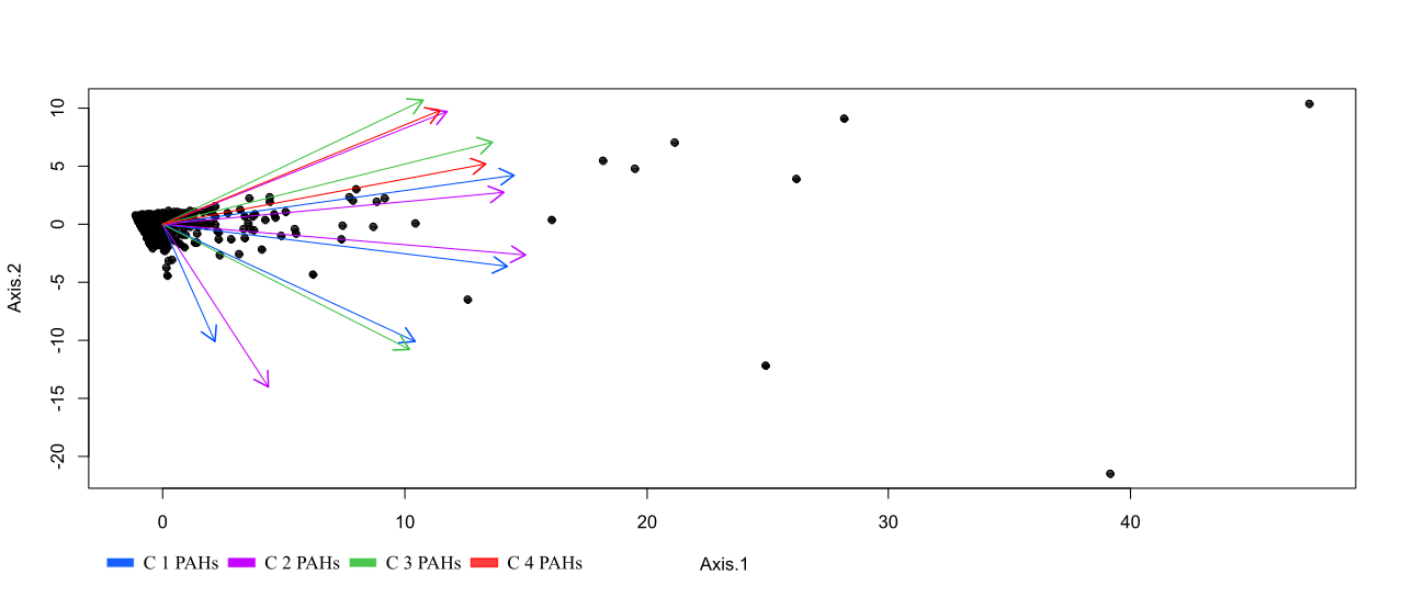
Figure 10. PCOA vectors of compound fractionation. Many C3, and both C4 PAH compounds trend nearly orthogonal to several C1-C2 hydrocarbons. As C2 and C3 hydrocarbons are intermediate molecular weights we see an expected overlap in these groups. Increased concentrations of lighter hydrocarbons are generally pyrogenic in nature while heavier C4 chains are typically petrogenic.
This analysis has been completed as part of the University of Alberta's Renewable Resources 690 - Multivariate Statistics For Environmental Sciences course. The raw data is publicly available from Alberta Environment and Parks. Analysis is preliminary and is not intended to inform management or policy directions. Neither the University of Alberta or Brandon Hill accept any risk of liability with the use or misuse of the analysis provided.
